Notes on the intro course from 3b1b.

I) vector basics

what’s a vector

physics: arrows in space, defined by length and direction and are movable
cs: ordered lists of numbers, i.e.
math: a mix of the above

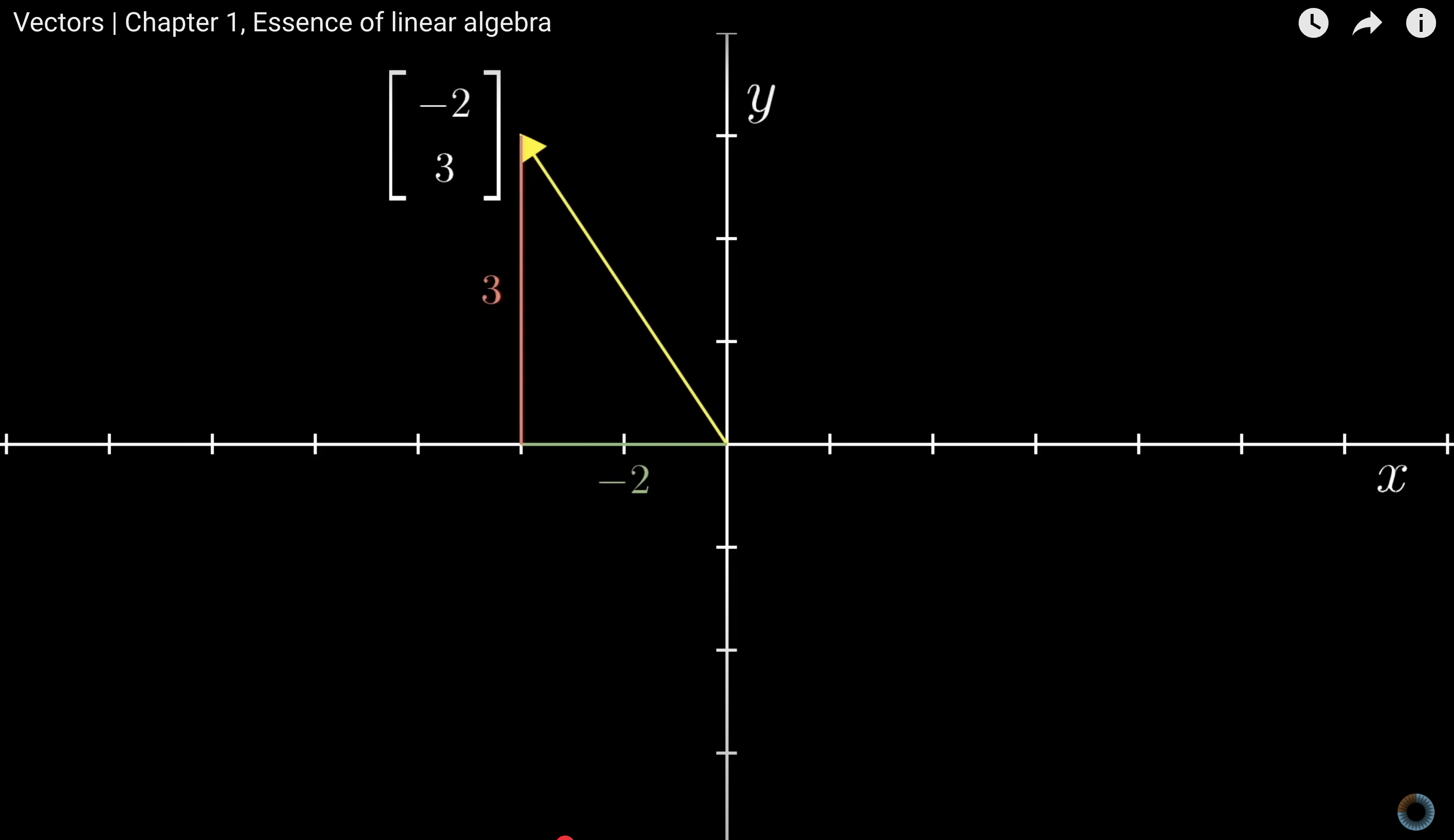
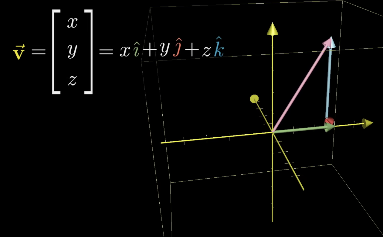
think about an arrow in a coordinate system, starting from the origin - 3b1b

fundamental vector operations

addition

each vectors is a step, a movement in space. First, walk , then .
this is the same as walking to start with!

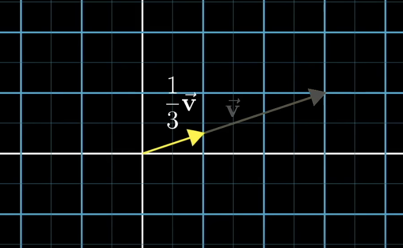
multiplying by a scalar

scaling: stretching, squishing, reversing direction.
scalar: number

Conclusion

it doesn’t matter whether we fundamentally see a vector as a list of numbers or an arrow in space. What matters is that we can translate between them.

II) linear combinations, span, basis

: unit vector in x direction
: unit vector in y direction
so what is ? Just the scaled and , i.e.
and are the basis of the coordinate system. We could have chosen a different one!
is a linear combination of those two vectors
the span of the two vectors and is the set of all their linear combinations!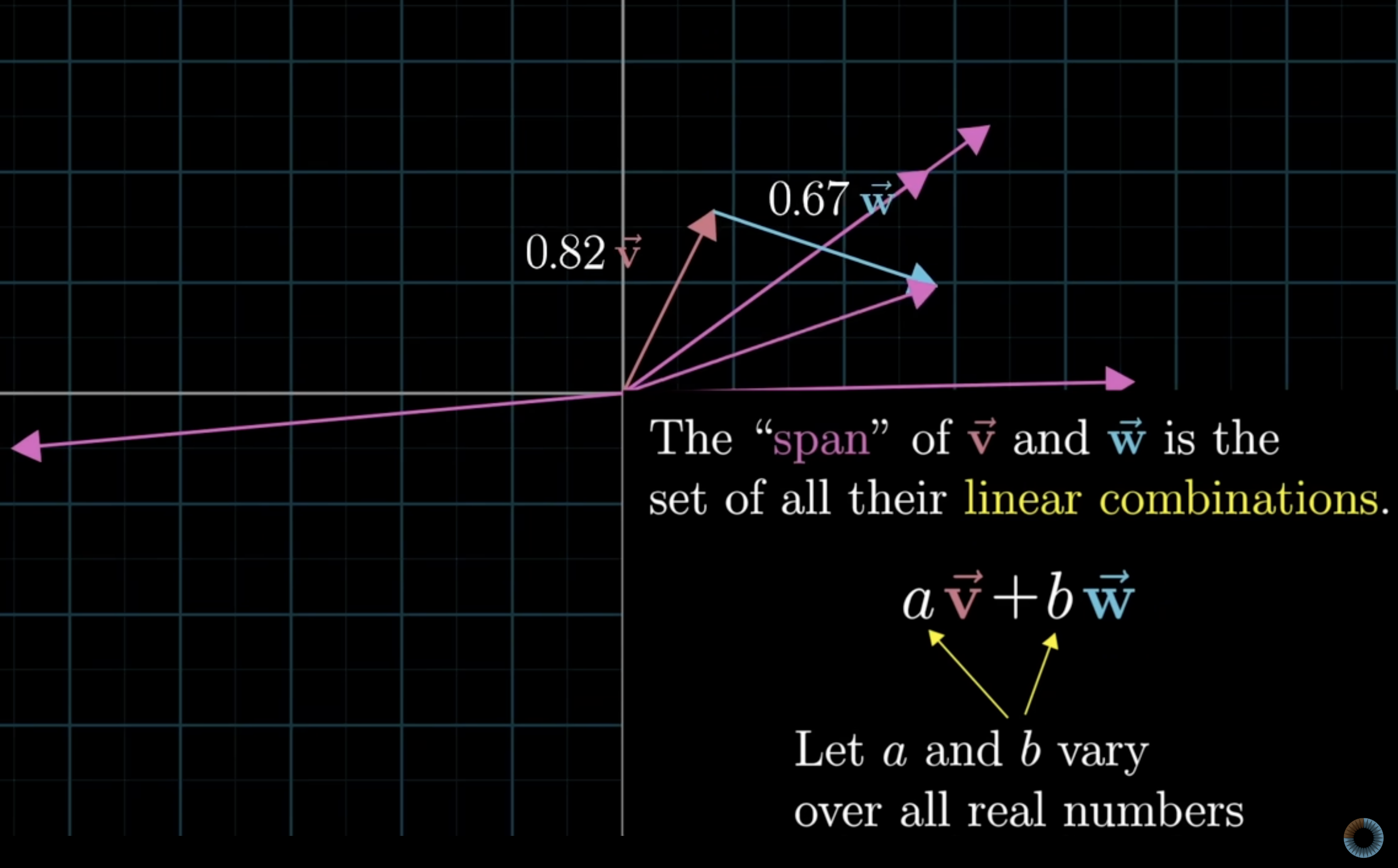
iow: the span consists of all vectors that can be expressed as a weighted sum of the original vectors, with weights being scalars.
- in 2d, the span covers the whole plane, except the two vectors are 0 or point in the same direction (then the span covers the line along which they’re pointing)
- in 3d, the span of the two vectors is a flat sheet going through 3d space
- ~ in 3d, the span of three vectors covers 3d space, except some of the vectors are linearly dependent
- if a vector adds a new dimension to the span, they are linearly independent

technical definition of basis:

the basis of a vector space is a set of linearly independent vectors that span that space

linearly independent + span the space
if not linearly independent, there’d be redundancy, one could just remove a vector
if not spanning the space, they couldn’t form a basis as not all vectors could be expressed
linear independence ensures uniqueness of the representation of a vector in space
for an n-dimensional vector space, any basis will contain exactly n vectors

III) Linear transformations and matrices

Linear transformation

transformation ~ function
linear ~ lines remain lines, origin remains fixed (in 2d)
linear ~ keeping gridlines parallel and evenly spaced

think: arrow a moving into arrow b as a transformation. Then, all arrows moving at once! now: vectors as points, not arrows

How to describe a linear transformation numerically?

Note

we only need to record where the basis vector and land, everything else goes from there

So more generally, let’s say we know where the basis vectors land:

now where does an arbitrary vector land?

so we can say where any vector lands using this formula!

Note

a 2d linear transformation is completely described by 4 numbers, the two coordinates where lands and the two coordinates where lands!

it’s common to package these coordinates into a 2x2 Matrix, where the columns are where lands and where lands!

Now this (middle bit, it’s a sum of scaled vectors!) gives us the intuition for matrix vector multiplication, no need to memorise.

Some insights:

if the vectors that and land on are linearly dependent, the 2d space collapses into a 1d line

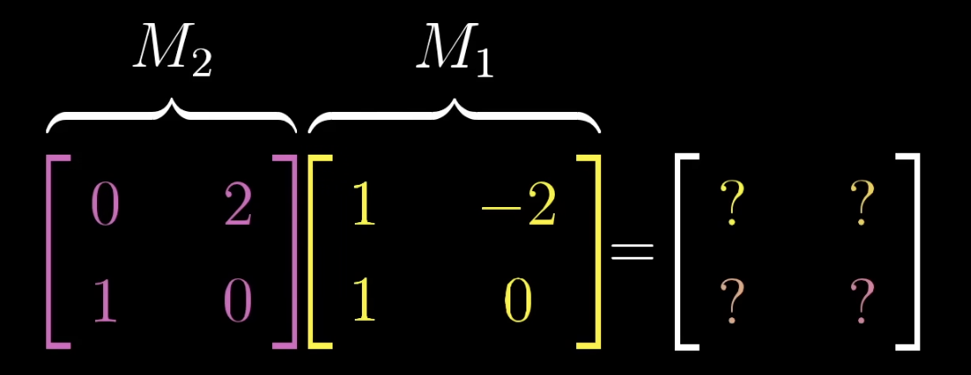
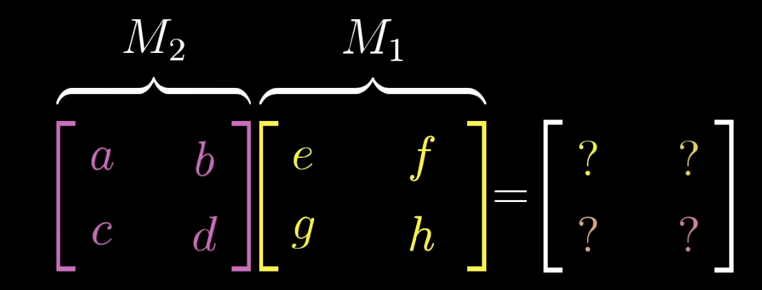
IV) Matrix multiplications as composition

Composition: two linear transformations in a row, like a rotation and a shear. There will be a matrix which represents the rotation, a matrix which represents the shear, and a matrix which represents both together. The latter is where and end up after both transformations.

The composition is therefore the product of the shear and the rotation matrix.

How to read : right to left, first rotation, then shear. Comes from function notation .

So how to do matrix multiplication with our knowledge so far?

after the transformation lands on , lands on .
where lands after the transformation:
where lands after transformation:
now just put the two together to get the composite:

Now the general solution, without memorizing:

after the transformation, lands on
now where does land after the transformation? . Just a recap why that is: It’s because and just scale where the basis mors land (which is and ). This is because the resulting mor is linearly dependent.
now where does land after the transformation?
then, we can just take those together as the first and second column of the composition matrix:

What does matrix multiplication really represent?

Applying one transformation after another.

What this helps with, for example:

Is ? No! when thinking about one transformation, then the next, it becomes clear that it matters which transformation comes first.
Is matrix multiplication associative? ?
- if one thinks in transformations, would be first C, then B, then A. The same is true for , which is first C, then B, then A! Easy cheesy.

V) 3D linear transformation

same as before, but three basis vectors, , ,
how big is the matrix describing the transformation now? 3x3!
again two transformations

VI) The determinant

First intuition: The determinant is how much a linear transformation scales space.

scales the initial area of the unit square (1) to an area of 6, so the determinant is 6.
any area can be approximated by grid squares

Special cases

the determinant is 0 when it squishes space onto a line, i.e. a smaller dimension!
the determinant is negative, when the orientation of space has been flipped / inverted
- what does inverting mean? in 2d, it means that if is initially left of and after the transformation it’s right!
3D: now we’re scaling volume, not area. A determinant of 0 would mean squashing into 2d, a line, or even a single point. In that case, the columns of the determinant are linearly dependent.

Compute the determinant

Why?

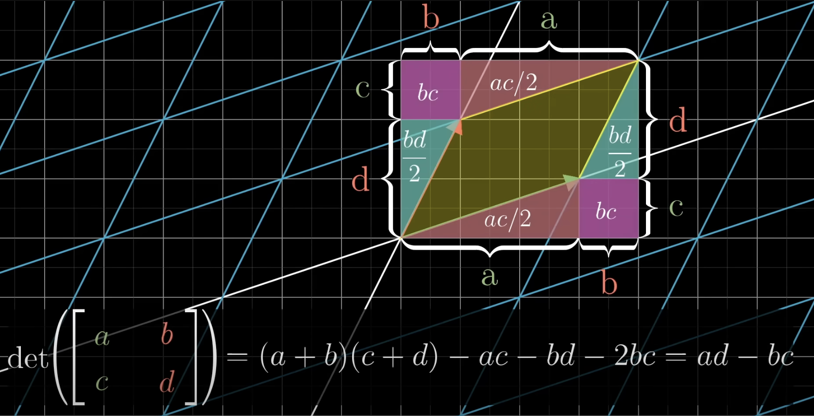
no really good intuition for the formula! But the essence is what the determinant really means.

Insight: Why is ?

after thought: determinants are all about how areas change due to a transformation

VII) Inverse matrices, column space and null space

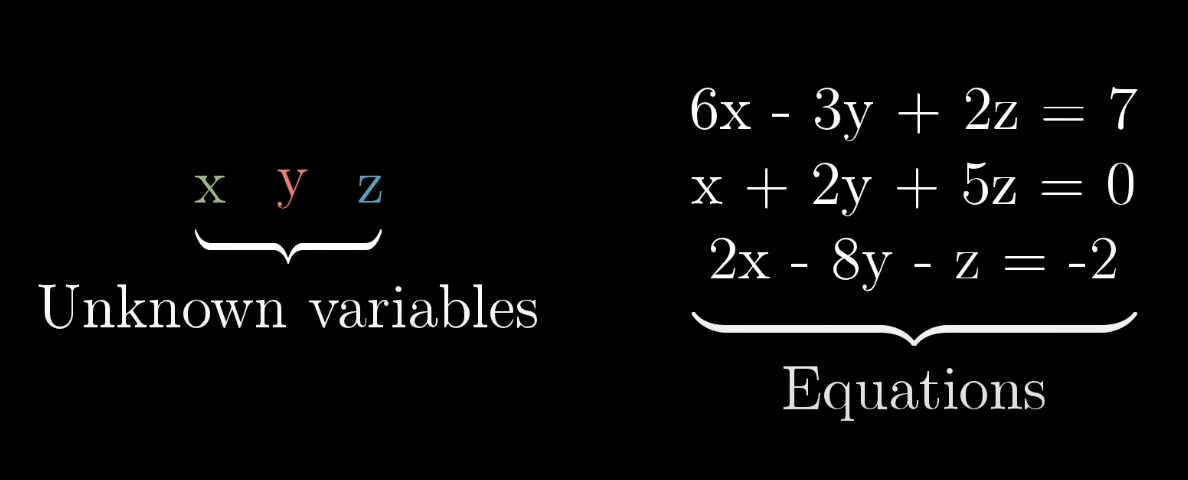
linear algebra let’s us solve systems of equations
to actually solve this: Gaussian elimination / row echolon form

linear system of equations

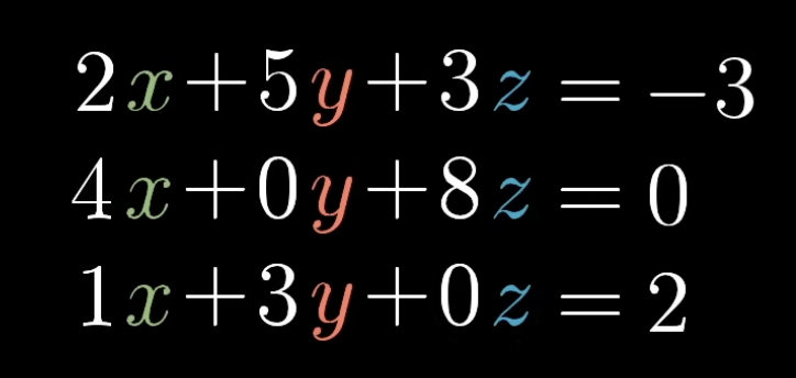Note: throw in 0 coefficients to nicely align x, y, z

This can be re-written as matrix vector multiplication!

Process to solve for in

Either we think about all these equations and variables, or …

… we’re simply looking for a vector , which after applying the transformation lands on !

We need to know whether the transformation squishes space on to a line / point or not: a)
b)
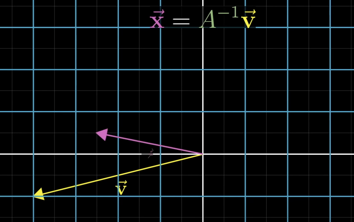
When , there will be one, and only one vector that lands on .
1. follow the transformation in reverse: where does go when going backwards?
2. we need the inverse of . E.g. if does a clockwise 90 degree rotation, then does a counterclockwise 90 degree rotation, ending up in the same spot!
3. (in the 2d case, the matrix is the identity matrix)
4. We can just multiply by the inverse matrix:
5. Geometrically, this means playing the transformation in reverse, following
6. It’s the most common case that there’s a unique solution. Like when we have as many equations as unknowns that’s often the case.
7. so, when then an inverse transformation exists.
8. when you first do and then it’s geometrically the same as doing nothing
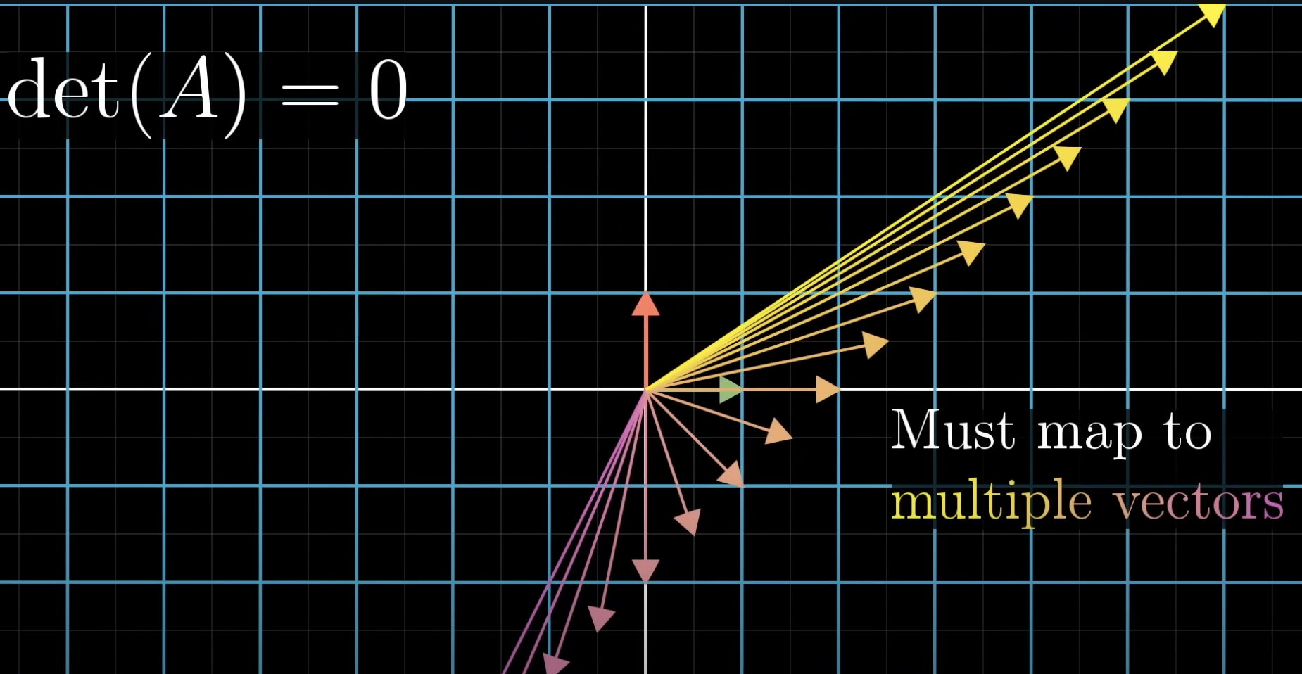
When and the transformation squishes space into a smaller dimension, there is no inverse !
1. there is no function to turn a line into a 2d plane! That’s because functions always map a single input to a single output. Here, we would need to map a single point to multiple vectors.
2. is there still a solution to ? Only when the vector lives somewhere on the squished space (like on the line in the 2d case). So solutions can still exist when the determinant is 0!

New terms

Column space: the span (all possible linear combinations) of the column vectors of a matrix.
Rank: number of dimensions in the column space
- Full rank: dimensions = n(columns)
- zero rank is always included, as linear transformations keep origin fixed
- Null space or Kernel : when space is squished, many vectors land on the origin

Note

when we have a linear system we can solve for using the inverse matrix through multiplying : , which is .
inverse matrices are needed to solve all sorts of things from linear regression to gp’s, but matrix inversion has O(n^3) complexity, so usually something else is taken such as Cholesky
the idea of column space let’s us figure out whether a solution even exists
null space can tell us what possible solutions can look like

Still don’t know: what actually is the null space and why is it important?

VIII) Dot products and duality

numeric

geometric dot product of vectors and is projecting onto and then multiplying the length of projected with the length of

dot product negative when vectors are pointing in opposite directions
dot product is zero when vectors are perpendicular
order doesn’t matter!

Why does the numeric calculation have anything to do with projection?

Duality

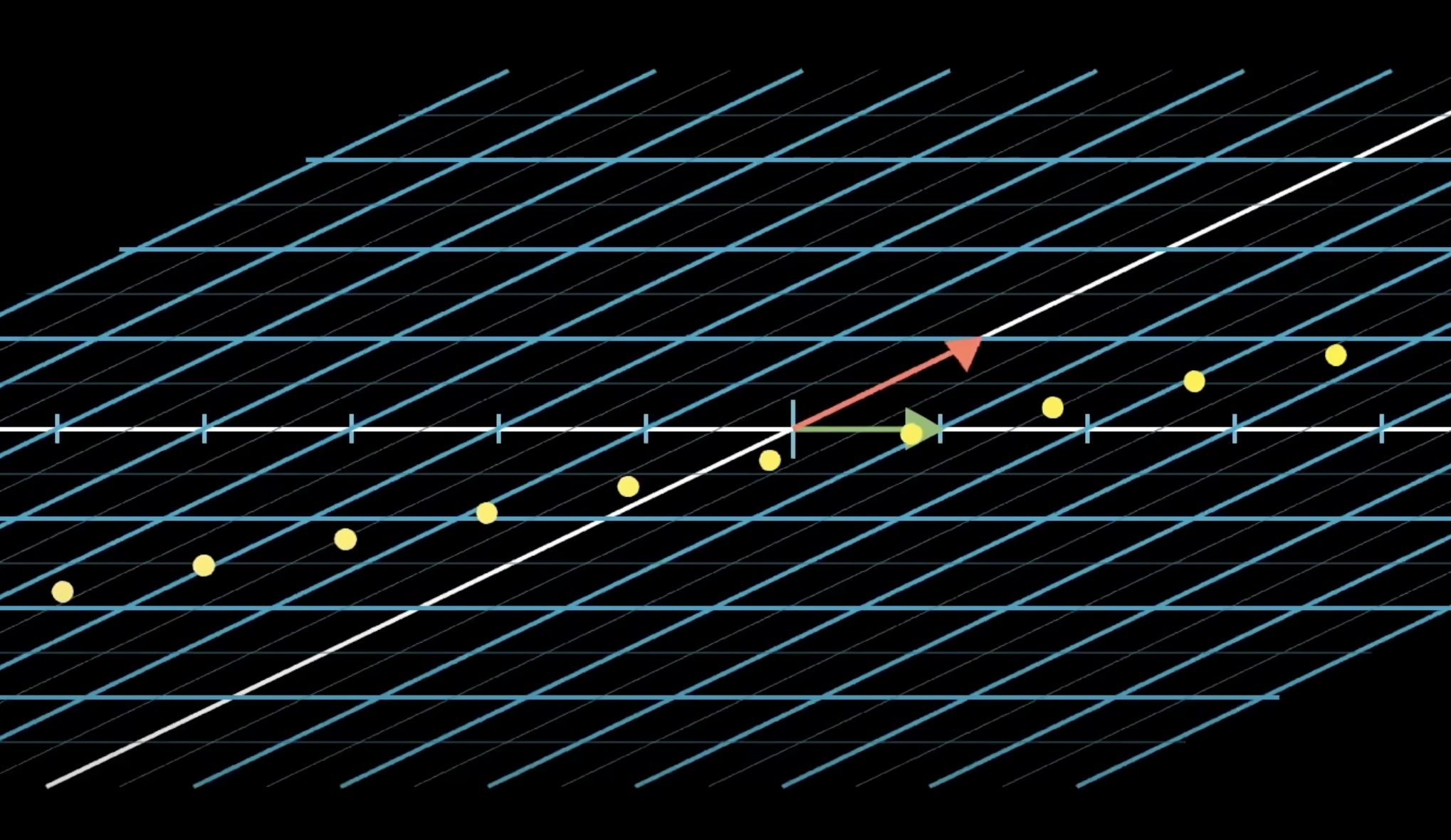
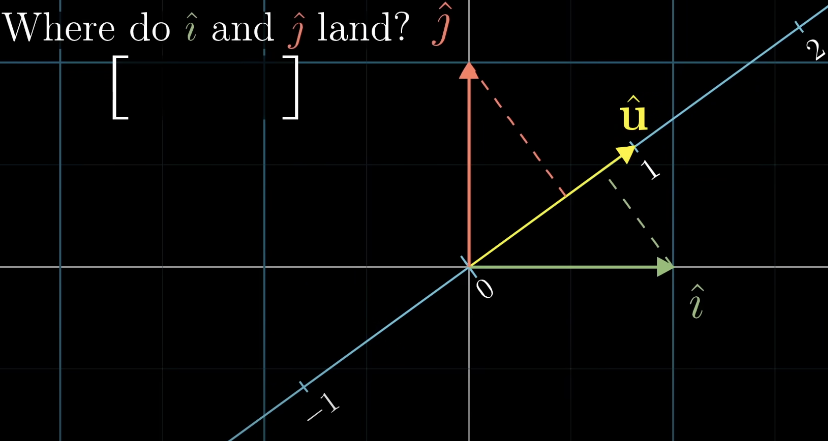
Let’s think about a linear transformation from from multiple to one dimension (number line).
When you take a line in two dimensions and project them onto the number line, the dots are evenly spaced (still).
and just each land on a number

let’s say the transformation is , here lands on 1 and lands on 2
where does get projected on?
multiplying a 1 x 2 matrix by a vector feels like taking the dot product!
there’s an association between 1 x 2 matrices and 2d vectors. The 1 x 2 matrix is a like a vector tipped on it’s side.
a linear transformation (2 x 1 matrix) that takes vectors to numbers is the dual of vectors themselves?
there’s a connection between linear transformations that take vectors to numbers, and vectors themselves

Let’s think this through.

We imagine a number line going through 2d space, and a sitting in 2d space, but happening to be the unit vector on the number line.
now we project 2d vectors onto the number line (linearly). The outputs of this function are numbers, not 2d vectors.

what’s the projection matrix?

symmetry: projecting onto is symmetric to projecting onto !
projecting onto the x-axis is just the x coordinate of
so lands on the number line on the number that’s the x-coordinate of and lands on the number line on the number that’s the y-coordinate of ! Very cool

Note

For any 2d-to-1d linear transform, say , there’s a unique vector which corresponds to that transformation. Hence applying that transformation is the same as taking the dot-product with that vector. That’s duality!

Summary: The dot product is an interesting tool to understand projections, and whether two vectors point in the same direction!

IX) Cross products

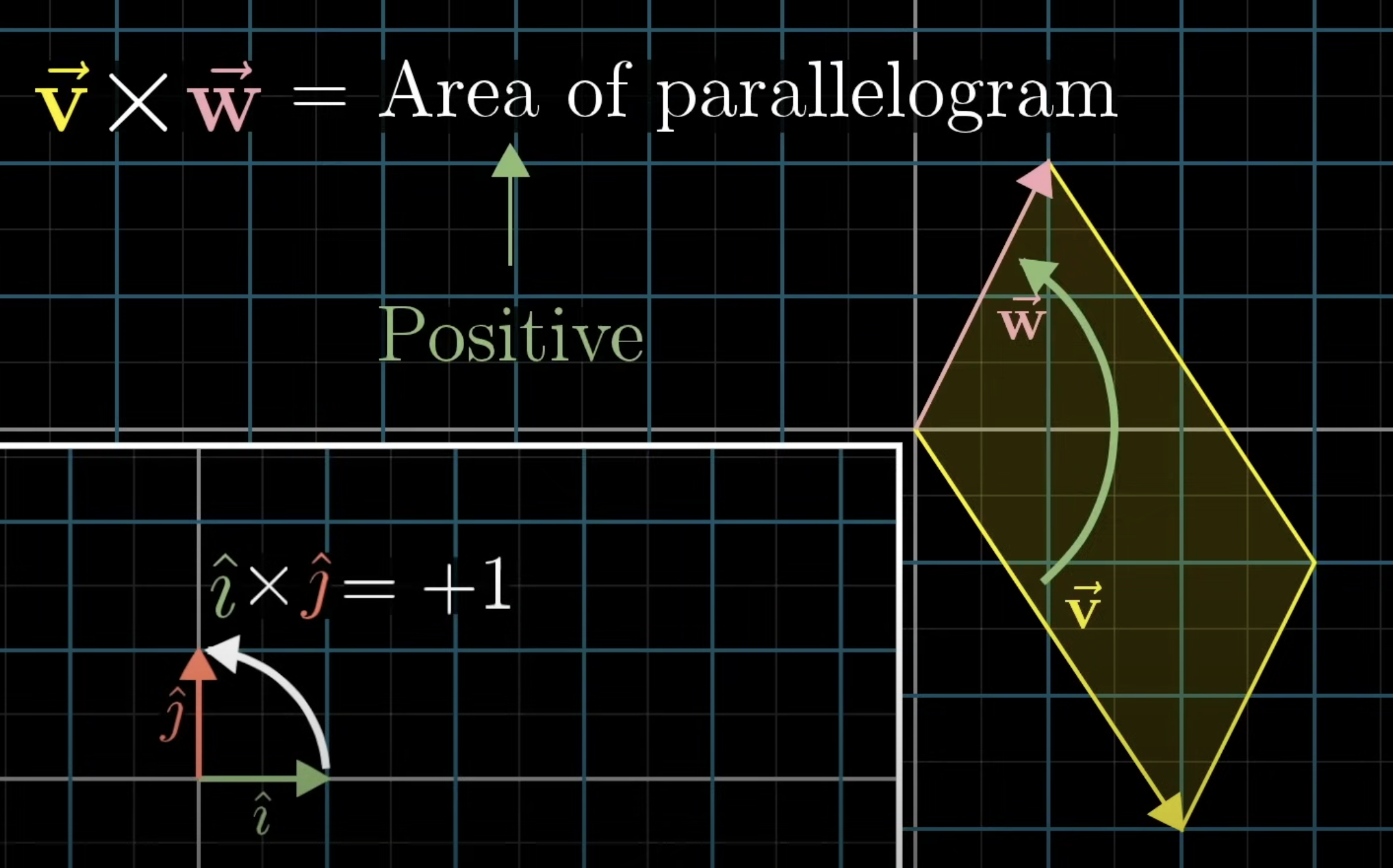
the cross product is equal to the area of the parallelogram of and .
it’s positive if is on the right of .
to remember this: The cross product of the basis vectors = +Area of parallelogram because is on the right of (this is what defines it)
if is on the left of , then = -Area of parallelogram
hence, order matters!
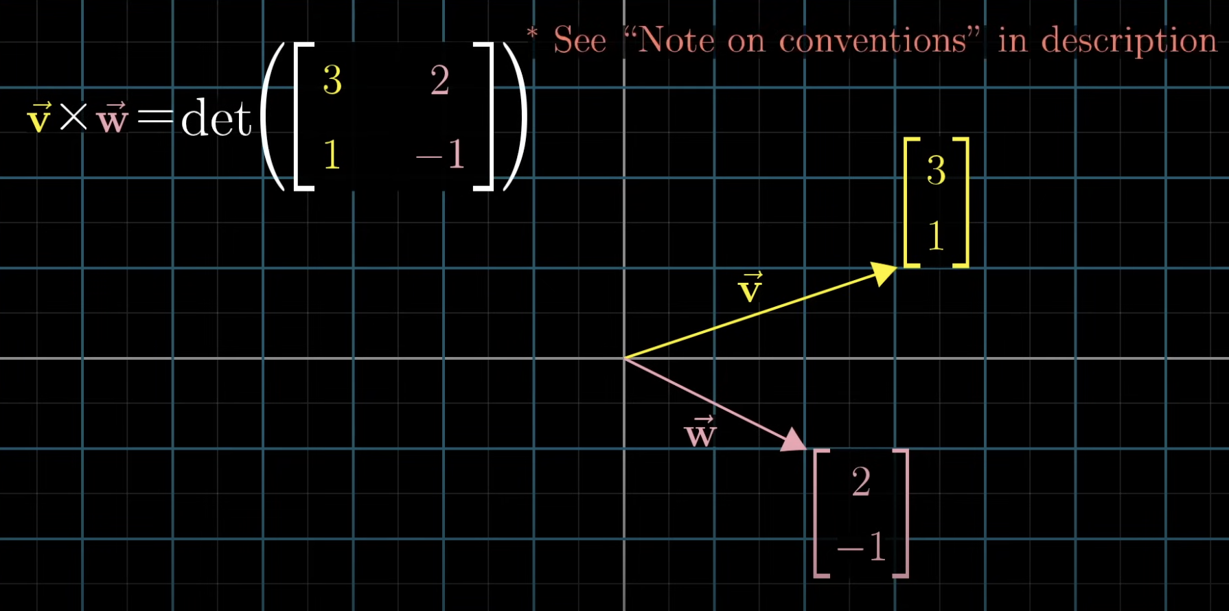
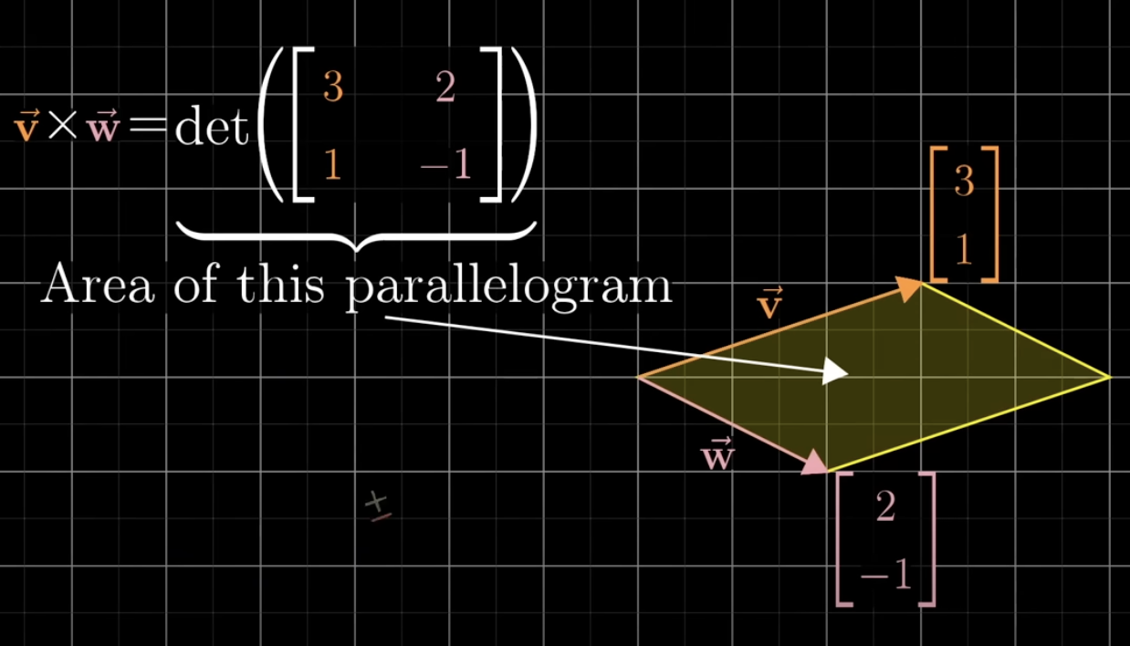
To compute the cross product , we stack both vectors into a matrix and calculate the determinant!
This works because determinants are about how areas change due to transformation (what the matrix represents)

all the above are technically not the cross product!

The actual output of the cross product is a vector with a length equal to the area of the parallelogram, which goes perpendicular to the parallelogram! But which way? → check right hand rule

Process of computing the cross product:

= =

this is a bit weird. Why are the basis vectors entries in that matrix?
the result is the vector that’s as long as the area of the parallelogram, and which is perpendicular to it, obeying the right hand rule

X) Cross Products in the light of linear transformation

recap: whenever we have a linear transformation from any space onto the number line * the transformation is described by 1-row matrix (telling us where each basis vectors land) * and there’s a vector in the original space that is the dual of that matrix … * where the transformation is the same as taking a dot product with that vector!

The cross product is a slick example of this!

2D cross product:

line up vectors colwise
calc determinant
equals area of the parallelogram

3D cross product

doesn’t actually take in three vectors and spits out a number
instead takes two 3D vectors and spits out a vector
but it’s not too far, let’s imagine instead of three fixed vectors, let the first vector be three variables
for a given vector , consider the parallelepiped between that vector and and (which is the determinant)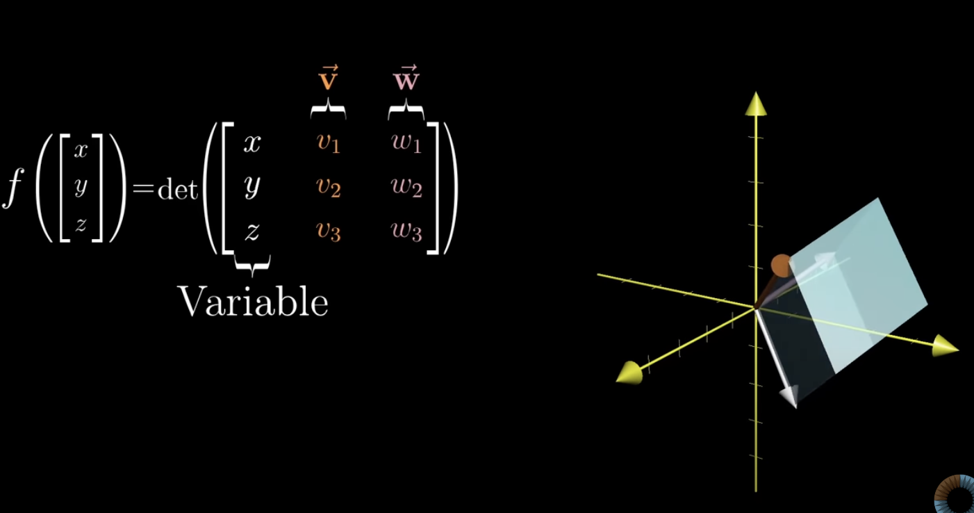
this function is linear, there is a way to describe it as matrix multiplication
it goes from three to one dimension
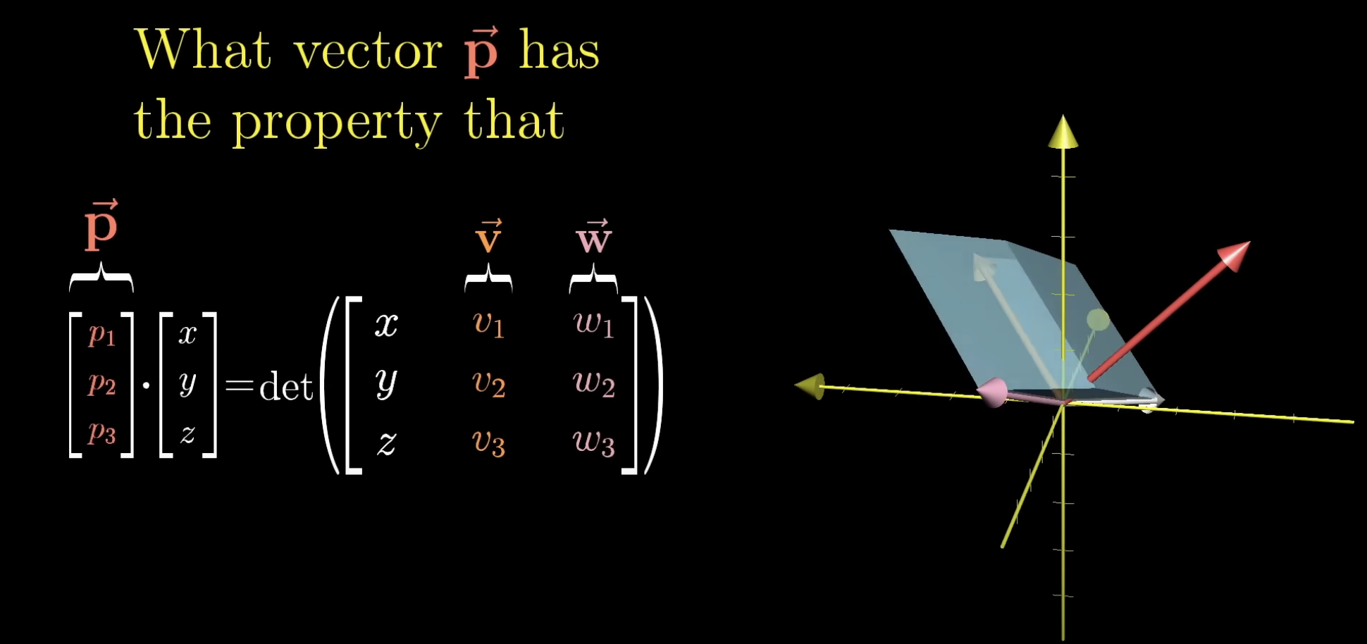
⇒ 1 x 3 matrix encodes this!
now we’ve got duality, so the 1x3 matrix is a vector
so now we can think about dot products again
the dual vector is a vector that is perpendicular to and and a length equal to the area of the parallelogram spanned by the two vectors TODO: revisit this video

XI) Cramers rule

how to solve linear equations
the challenge: finding the input vector that lands on the output vector after the linear transformation

What we know: The output vector is some linear combination of the columns of the matrix and , i.e. . Now there are two cases:

Case 1: The determinant is zero and the transformation squishes space into a lower dimension. In that case, either no vector lands on the output vector , or a whole lot of vectors do!

Case 2: The determinant is not zero.

the outputs then still span the full n-dimensional space. Every input lands on one output, and every output has only one input.

Though experiment: dotting with the basis vectors gives x and y.

Before transformation: and same for the y component. Then, is transformed ?? answer is no, dot product before and after transformation will usually be very different.
But if they preserve dot products, they are called orthonormal
solving a system with an orthonormal matrix is easy

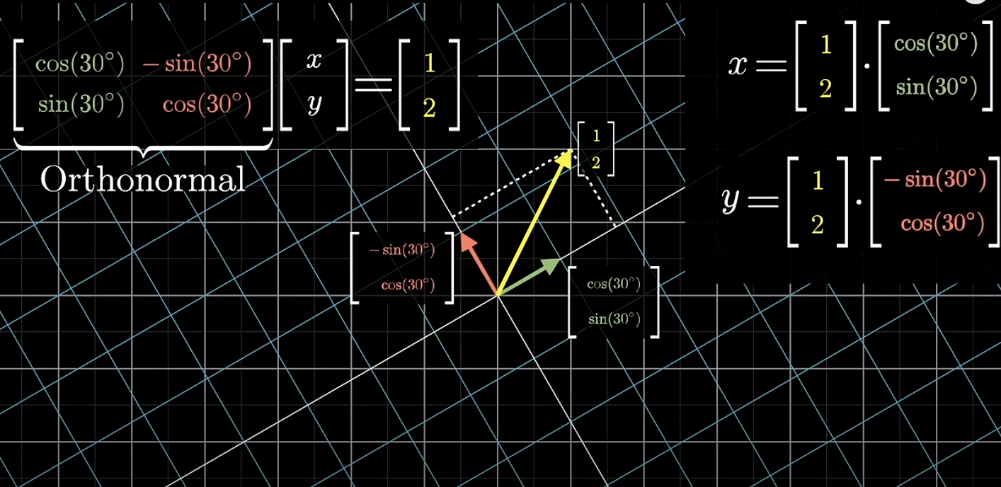
This is a very special case, but think: is there an alternate geometric understanding for the coordinates for our input vector that remains unchanged after transformation?

TODO: watch again

XII) Change of basis

and are basis vectors
any vector’s coordinates are scalars as they scale the basis vectors
e.g. is and like so:
there can be alternative basis vectors though
so the same vector could be something else in a different coordinate system (but it would still be defined as scaling the basis vectors)
the origin is always though, the thing you get when scaling a vector by 0
how to translate between coordinate systems?

Let’s say we have a different coordinate system with basis vectors and . We can then look at what the coordinates of these basis vectors are in ‘our’ coordinate system and just scale them. A vector in that coordinate system would be a vector in our coordinate system, see here:

This is just matrix vector multiplication, where the matrix columns are the alternative basis vectors and the vector is what we want to translate into the alternative coordinate system!

Fantom Filters

essence of linear algebra

I) vector basics

what’s a vector

fundamental vector operations

addition

multiplying by a scalar

II) linear combinations, span, basis

technical definition of basis:

III) Linear transformations and matrices

IV) Matrix multiplications as composition

So how to do matrix multiplication with our knowledge so far?

Now the general solution, without memorizing:

V) 3D linear transformation

VI) The determinant

Special cases

Compute the determinant

VII) Inverse matrices, column space and null space

linear system of equations

VIII) Dot products and duality

Why does the numeric calculation have anything to do with projection?

IX) Cross products

X) Cross Products in the light of linear transformation

XI) Cramers rule

XII) Change of basis

Graph View

Table of Contents

Backlinks